optimize
Numerical optimisation and root finding in pure Go (CGO=0): minimisation, scalar and system roots, nonlinear least squares, curve fitting with parameter covariance, and linear programming.
The package covers the parts of scipy.optimize that scientific notebooks use
most. Each function documents the SciPy call it corresponds to. The test suite
replays SciPy 1.18.1 on standard problems, and it checks solutions, objective
values, status codes, messages, and iteration and evaluation counts.
go get github.com/go-numerics/optimize@v0.1.0It works with go-ndarray: curve-fit
data, covariances and LP constraint matrices are *ndarray.Array, and results
have …Array() accessors.
What is there
| Go | SciPy | Algorithm |
|---|---|---|
Minimize(p, x0, NelderMead, opts) | minimize(method='Nelder-Mead') | downhill simplex, adaptive option, bounds |
Minimize(…, Powell, …) | minimize(method='Powell') | conjugate directions, bounds |
Minimize(…, CG, …) | minimize(method='CG') | Polak–Ribière+, strong Wolfe |
Minimize(…, BFGS, …) | minimize(method='BFGS') | inverse-Hessian BFGS, O(n²) update |
Minimize(…, NewtonCG, …) | minimize(method='Newton-CG') | truncated Newton (Hess, HessP or FD) |
Minimize(…, LBFGSB, …) | minimize(method='L-BFGS-B') | L-BFGS-B 3.0 with bounds |
MinimizeScalar, Fminbound, Bracket | minimize_scalar (brent, golden, bounded), fminbound, bracket | Brent, golden section, FMIN |
Brentq, Brenth, Ridder, Bisect, Newton, RootScalar | brentq, brenth, ridder, bisect, newton (Newton/secant/Halley), root_scalar | |
Root, Fsolve | root(method='hybr'), fsolve | MINPACK hybrd/hybrj (Powell hybrid) |
LeastSquares(…, TRF, …) | least_squares(method='trf') | trust-region reflective, bounds, robust losses, x_scale |
LeastSquares(…, LM, …), Leastsq | least_squares(method='lm'), leastsq (with cov_x) | MINPACK lmder/lmdif |
CurveFit, CurveFitModel | curve_fit (sigma 1-D/2-D, absolute_sigma, bounds, losses) | LM or TRF, covariance as SciPy |
Linprog | linprog | revised simplex (default) or interior point; duals |
Brute | brute | grid then Nelder–Mead polish |
CheckGrad, ApproxFprime | check_grad, approx_fprime | forward differences |
Gradients are optional everywhere. Without one, finite differences use the
step rules of SciPy’s approx_derivative, kept inside the bounds.
Non-convergence is reported in Success/Status/Message as SciPy does.
Invalid input returns an error.
Examples
Each example below is a runnable, output-checked Go example in
example_test.go, and its output was checked against SciPy.
// scipy.optimize.minimize(rosen, x0, jac=rosen_der, method='BFGS')
r, err := optimize.Minimize(optimize.Problem{Func: rosen, Grad: rosenDer},
	[]float64{-1.2, 1}, optimize.BFGS, nil)
// r.X = [1 1], r.Nit = 32 (SciPy: 32), "Optimization terminated successfully."

// scipy.optimize.minimize(f, x0, method='L-BFGS-B', bounds=[(-2, 0.5), (None, None)])
r, _ = optimize.Minimize(optimize.Problem{Func: f}, []float64{0, 0}, optimize.LBFGSB,
	&optimize.Options{Bounds: []optimize.Bound{{Lo: -2, Hi: 0.5}, optimize.Unbounded()}})

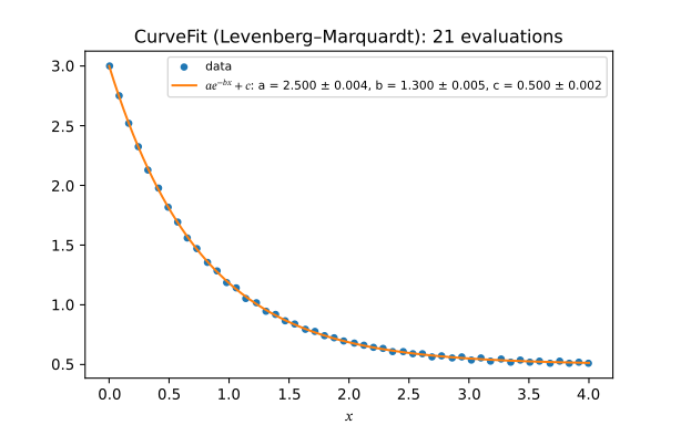
// popt, pcov = scipy.optimize.curve_fit(lambda x, a, b, c: a*np.exp(-b*x) + c, x, y)
fit, err := optimize.CurveFit(func(x float64, p []float64) float64 {
	return p[0]*math.Exp(-p[1]*x) + p[2]
}, xdata, ydata, []float64{1, 1, 1}, nil)
// fit.Popt, fit.PcovArray(), fit.Perr()  ->  a = 2.500 ± 0.004, b = 1.300 ± 0.005, c = 0.500 ± 0.002

// scipy.optimize.brentq(lambda x: x**3 - 2*x - 5, 2, 3)
root, _ := optimize.Brentq(func(x float64) float64 { return x*x*x - 2*x - 5 }, 2, 3, nil)
// root.Root = 2.094551481542…, 7 iterations (as SciPy)

// scipy.optimize.root(fun, [0, 0])        (fun writes f(x) into its second argument)
sol, _ := optimize.Root(optimize.SystemProblem{Func: fun}, []float64{0, 0}, nil)

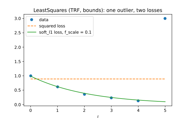
// scipy.optimize.least_squares(fun, x0, bounds=([0, 0], [2, 0.5]), loss='soft_l1', f_scale=0.1)
ls, _ := optimize.LeastSquares(optimize.LSProblem{Func: resid, M: m}, []float64{1, 0.1}, optimize.TRF,
	&optimize.LSOptions{Bounds: []optimize.Bound{{0, 2}, {0, 0.5}}, Loss: optimize.LossSoftL1, FScale: 0.1})

// scipy.optimize.linprog(c, A_ub=A, b_ub=b, bounds=[(None, None), (-3, None)])
lp, _ := optimize.Linprog([]float64{-1, 4}, optimize.LPConstraints{AUb: A, BUb: b,
	Bounds: []optimize.Bound{optimize.Unbounded(), {Lo: -3, Hi: math.Inf(1)}}}, nil)
// lp.X = [10 -3], lp.Fun = -22, lp.IneqLin.Marginals (HiGHS sign convention)
Callbacks receive the point first and write their outputs into the slices that
follow: Func(x), Grad(x, g), FuncGrad(x, g) (SciPy’s jac=True),
Hess(x, h), HessP(x, p, hp), residuals Func(x, f), Jacobians Jac(x, J).
Matrices are row-major []float64.
The README’s curve fit and robust least-squares examples, drawn with go-plot from the results they return:
package main

import (
	"fmt"
	"math"

	"github.com/go-ndarray/ndarray"
	"github.com/go-numerics/optimize"
	"github.com/go-plot/plot"
)

func init() { register("curvefit", curvefit) }

// The README's CurveFit example: 50 points of 2.5 exp(-1.3x) + 0.5 with a
// deterministic ripple, fitted from p0 = (1, 1, 1). The legend prints the
// parameters and standard errors CurveFit returned.
func curvefit() *plot.Figure {
	x, _ := ndarray.Linspace(0, 4, 50)
	y := x.Map(func(v float64) float64 { return 2.5*math.Exp(-1.3*v) + 0.5 + 0.01*math.Sin(37*v) })
	model := func(x float64, p []float64) float64 { return p[0]*math.Exp(-p[1]*x) + p[2] }
	r, err := optimize.CurveFit(model, x, y, []float64{1, 1, 1}, nil)
	if err != nil {
		panic(err)
	}
	perr := r.Perr()
	xs := linspace(0, 4, 200)
	fit := make([]float64, len(xs))
	for i, v := range xs {
		fit[i] = model(v, r.Popt)
	}
	fig, axs := plot.Subplots(1, 1, plot.FigSize(6.4, 4))
	ax := axs[0][0]
	ax.Plot(x, y, plot.Marker("o"), plot.LineStyle("None"), plot.MarkerSize(4), plot.Label("data"))
	ax.Plot(xs, fit, plot.Label(fmt.Sprintf(`$a e^{-bx} + c$: a = %.3f ± %.3f, b = %.3f ± %.3f, c = %.3f ± %.3f`,
		r.Popt[0], perr[0], r.Popt[1], perr[1], r.Popt[2], perr[2])))
	ax.SetTitle(fmt.Sprintf("CurveFit (Levenberg–Marquardt): %d evaluations", r.Nfev))
	ax.SetXLabel(`$x$`)
	ax.Legend(plot.FontSize(8))
	return fig
}
package main

import (
	"math"

	"github.com/go-numerics/optimize"
	"github.com/go-plot/plot"
)

func init() { register("robust", robust) }

// The README's LeastSquares example, fitted twice: with the ordinary squared
// loss, which the outlier at t = 5 drags upwards, and with soft_l1, which
// keeps it from dominating. Same bounds, same start.
func robust() *plot.Figure {
	t := []float64{0, 1, 2, 3, 4, 5}
	y := []float64{1.0, 0.62, 0.36, 0.23, 0.13, 3.0} // the last point is an outlier
	p := optimize.LSProblem{M: len(t), Func: func(x, f []float64) {
		for i := range t {
			f[i] = x[0]*math.Exp(-x[1]*t[i]) - y[i]
		}
	}}
	bounds := []optimize.Bound{{Lo: 0, Hi: 2}, {Lo: 0, Hi: 0.5}}
	linear, err := optimize.LeastSquares(p, []float64{1, 0.1}, optimize.TRF,
		&optimize.LSOptions{Bounds: bounds})
	if err != nil {
		panic(err)
	}
	soft, err := optimize.LeastSquares(p, []float64{1, 0.1}, optimize.TRF,
		&optimize.LSOptions{Bounds: bounds, Loss: optimize.LossSoftL1, FScale: 0.1})
	if err != nil {
		panic(err)
	}
	xs := linspace(0, 5, 200)
	curve := func(x []float64) []float64 {
		v := make([]float64, len(xs))
		for i, s := range xs {
			v[i] = x[0] * math.Exp(-x[1]*s)
		}
		return v
	}
	fig, axs := plot.Subplots(1, 1, plot.FigSize(6.4, 4))
	ax := axs[0][0]
	ax.Plot(t, y, plot.Marker("o"), plot.LineStyle("None"), plot.Label("data"))
	ax.Plot(xs, curve(linear.X), plot.LineStyle("--"), plot.Label("squared loss"))
	ax.Plot(xs, curve(soft.X), plot.Label("soft_l1 loss, f_scale = 0.1"))
	ax.SetTitle("LeastSquares (TRF, bounds): one outlier, two losses")
	ax.SetXLabel(`$t$`)
	ax.Legend()
	return fig
}
How close to SciPy
All numbers below are against SciPy 1.18.1 fixtures generated by
testdata/gen/*.py (run with uv run --with scipy --with numpy python …) and
embedded in the tests. They are the same on arm64 and amd64, except where
noted.
| Area | Fixtures | Result |
|---|---|---|
Minimize (NM, Powell, CG, BFGS, Newton-CG, L-BFGS-B) | 79 runs on Rosenbrock n=2/10/100, Beale, Himmelblau, Powell singular, Wood, with and without gradients, bounds, iteration limits | every converged SciPy run is matched with an objective at least as good, within the method’s own tolerance; on the arithmetic-only problems, 36/38 runs take SciPy’s exact path (identical nit, nfev, njev); the 2 exceptions are explained in docs/design.md |
| L-BFGS-B | 44 runs, including 8 problems that reach rare branches (Cholesky failures, the 3.0 backtrack, Cauchy breakpoints) | identical nit/nfev/njev/status/message on every analytic-gradient run except Rosenbrock n=100 (513 vs 514 iterations, SciPy’s Accelerate BLAS rounding); bit-identical to SciPy’s C code built with sequential BLAS |
Root/Fsolve | 23 runs (MGH problems with and without Jacobian, failure and option cases) | 23/23 identical counts, status and message; x bit-identical |
LeastSquares(LM) / Leastsq | 39 / 44 runs on the MGH least-squares set | 36/39 and 41/44 identical counts; the mismatches are on problems that call exp/sin/cos, where Go’s libm and the C library differ in the last ulp |
LeastSquares(TRF) | 89 runs: MGH problems, bounds, all robust losses, x_scale, 2-/3-point differences | 86/89 identical nfev/njev/status (84/89 on amd64); every cost and active mask matches |
CurveFit | 11 fits (exponentials, Gaussians, sum of two Gaussians, a 2-variable plane, 1-D and 2-D sigma, bounds, absolute_sigma, m = n) | popt within 1e-6, pcov within 1e-5 relative, identical nfev on every fit |
| Scalar roots | 71 runs on 11 hard functions (multiple roots, flat, steep, kinks, poles) × 7 methods | 68/71 on SciPy’s exact path (same root, iterations, calls); the rest differ only through cos/exp in the last ulp |
MinimizeScalar, Bracket | 36 + 6 runs | identical x/nit/nfev/message on arithmetic-only functions |
Linprog | 46 problems vs HiGHS: Klee–Minty, cycling examples, degenerate, free and upper-bounded variables, redundant rows, infeasible, unbounded, random up to 60×40 | 46/46 statuses; objective error ≤ 1.8e-15 (simplex) and ≤ 2e-8 (interior point); solutions and duals inside SciPy’s optimal sets |
Brute | 4 grids (the SciPy documentation example, Himmelblau, Rosenbrock 3-D) | x and f to 1e-9 |
How such close agreement is possible:
- The ports follow their references statement by statement.
- Every product that feeds an addition is rounded explicitly, because Go would otherwise fuse it into an FMA on arm64 and other architectures.
- The tests use FMA-free oracles.
See Design.
Negative controls. One algorithmic step was broken at a time; each break made the suite fail, and each was then reverted:
| Broken step | Failing tests |
|---|---|
| A term dropped from the BFGS update | 6 |
A sign flipped in Moré–Thuente’s dcstep | 57 |
| The wrong Brent golden constant | 4 |
The Levenberg correction dropped in lmpar | 40 |
A sign flipped in dogleg | 17 |
| TRF reflection disabled, or its radius growth changed | 20 / 48 of the 89 cases leave SciPy’s path |
| Max instead of min in the simplex ratio test | 83 |
| The sign of the interior-point corrector flipped | iteration parity drops from 43 to 2 of 46 |
| L-BFGS-B’s subspace backtrack skipped, its Cauchy f2 update dropped, or its breakpoint heap disabled | named fixtures fail for each |
Performance
Medians of 7 rounds, with Go and SciPy interleaved on a loaded host. Performance has the method and caveats.
| Benchmark | Go | SciPy | Speed-up |
|---|---|---|---|
| Rosenbrock n=2, BFGS | 5.7 µs | 2.58 ms | 449× |
| Rosenbrock n=100, BFGS | 14.8 ms | 87.9 ms | 5.9× |
| Rosenbrock n=2, L-BFGS-B | 126 µs | 1.47 ms | 11.7× |
| Rosenbrock n=100, L-BFGS-B | 6.36 ms | 23.2 ms | 3.7× |
curve_fit, 10⁴ points, LM | 4.13 ms | 2.78 ms | 0.67× (SciPy faster) |
curve_fit, 10⁴ points, TRF | 5.97 ms | 4.61 ms | 0.77× (SciPy faster) |
brentq | 0.27 µs | 8.6 µs | 32× |
Most of SciPy’s time on small problems is Python overhead around the callbacks. Even after subtracting SciPy’s time spent in its own callbacks, the Go algorithms remain 2–300× faster, depending on the problem.
On large vectorised curve fits SciPy is faster today. Its model call is one NumPy expression, and its MINPACK/LAPACK kernels are compiled C. Our model evaluation is at parity; the gap is in the solver’s workspace handling.
Not done
minimize: trust-constr, SLSQP, COBYLA/COBYQA, TNC, dogleg/trust-ncg and the other trust-region methods, and constraints other than bounds. For L-BFGS-B, thehess_invoperator is not provided.root/least_squares:rootmethods other thanhybr; theband/col_derivoptions; dogbox; the lsmr trust-region solver and sparse Jacobians.linprog: HiGHS-class performance, MILP, singleton-row presolve, crossover and sparse matrices.- Global optimisers: differential_evolution, basinhopping, shgo, dual_annealing.
Licence
BSD 3-Clause; see LICENSE.
Created on by tannevaled
Modified on by tannevaled