integrate
Numerical integration and ODE solvers in pure Go (CGO_ENABLED=0): adaptive
quadrature (QUADPACK), fixed and sample rules, multiple integrals, and initial
value problems with RK45, RK23, DOP853, Radau, BDF and automatic stiffness
switching — the functionality of scipy.integrate for the Go scientific
stack (go-ndarray, go-plot,
go-notebook), with the same algorithms, defaults and diagnostics.
go get github.com/go-numerics/integrate@v0.1.0Headline numbers
- Same algorithms, same paths. QUADPACK is ported from the netlib Fortran;
the ODE methods follow SciPy’s implementations step for step. Against SciPy
1.18.1, 116 of 124 fixture integrals take exactly SciPy’s subdivision path
(same evaluation count, value to 1e-12), and 110 of 120
solve_ivpruns of the ported methods take exactly SciPy’s steps (same nfev, steps, njev, nlu). The remaining differences are explained in Verification: roundoff-limited paths that depend on the last bit, and three integrals where SciPy’s C translation of QUADPACK departs from the Fortran and this port agrees with the Fortran. - Faster. 6–8× SciPy on
quad(3× without counting Python callbacks), 90–190× onsolve_ivp(RK45, DOP853, Radau, BDF; same step sequences), 8–16× onodeint/LSODA (Performance). - Verified. Fixtures from SciPy and mpmath, the netlib Fortran as a second
oracle, a negative control on the coefficients, 100 % statement coverage
with
-race, CI lanes on amd64, arm64, riscv64, loong64, ppc64le, s390x, 386 and arm.
From SciPy to Go
| SciPy | Go |
|---|---|
quad(f, a, b) | integrate.Quad(f, a, b, nil) |
quad(f, 0, np.inf) | integrate.Quad(f, 0, math.Inf(1), nil) |
quad(f, a, b, epsabs=0, epsrel=1e-12, limit=200) | Quad(f, a, b, &integrate.QuadOptions{EpsAbs: -1, EpsRel: 1e-12, Limit: 200}) |
quad(f, a, b, points=[c]) | Quad(f, a, b, &integrate.QuadOptions{Points: []float64{c}}) |
quad(f, a, b, weight="cos", wvar=w) (also "sin", infinite b) | Quad(f, a, b, &integrate.QuadOptions{Weight: integrate.WeightCos, Omega: w}) |
quad(f, a, b, weight="alg", wvar=(al, be)) ("alg-loga", "alg-logb", "alg-log") | Quad(f, a, b, &integrate.QuadOptions{Weight: integrate.WeightAlg, Alpha: al, Beta: be}) |
quad(f, a, b, weight="cauchy", wvar=c) | Quad(f, a, b, &integrate.QuadOptions{Weight: integrate.WeightCauchy, C: c}) |
IntegrationWarning (ier 1–5, 7) | *integrate.QuadError returned with the result; errors.Is(err, integrate.ErrRoundoff) … |
dblquad(f, a, b, gfun, hfun) | integrate.DblQuad(f, a, b, gfun, hfun, nil), constants as integrate.Const(v) |
tplquad(f, a, b, g, h, q, r) | integrate.TplQuad(f, a, b, g, h, q, r, nil) |
nquad(f, ranges, opts=...) | integrate.NQuad(f, ranges, &integrate.NQuadOptions{...}) |
fixed_quad(f, a, b, n=5) | integrate.FixedQuad(f, a, b, 5) |
romberg(f, a, b) (SciPy < 1.15) | integrate.Romberg(f, a, b, nil) |
trapezoid(y, x), simpson(y, x=x), cumulative_trapezoid(y, x, initial=0), romb(y, dx) | Trapezoid(y, x, 0), Simpson(y, x, 0), CumulativeTrapezoid(y, x, 0, true), Romb(y, dx); TrapezoidND, SimpsonND, CumulativeTrapezoidND take an *ndarray.Array and an axis |
solve_ivp(fun, (t0, tf), y0) | integrate.SolveIVP(f, [2]float64{t0, tf}, y0, nil) |
method="Radau", rtol=1e-6, atol=[...], max_step, first_step, jac | &integrate.IVPOptions{Method: integrate.Radau, RTol: 1e-6, ATolVec: []float64{...}, MaxStep: …, FirstStep: …, Jac: …} |
t_eval=ts, dense_output=True, sol.sol(t) | TEval: ts, DenseOutput: true, sol.Sol.Eval(t) |
events=[g] with g.terminal = True, g.direction = -1 | Events: []integrate.Event{{F: g, Terminal: 1, Direction: -1}} |
sol.t, sol.y, sol.t_events, sol.nfev | sol.T, sol.Y (sol.YArray() for SciPy’s n × len(t) ndarray), sol.TEvents, sol.NFev |
odeint(func, y0, t, tfirst=True) | integrate.Odeint(f, y0, t, nil) → len(t) × n *ndarray.Array and an info record |
A right-hand side writes its derivative instead of returning it:
// SciPy: def lotka(t, y): return [1.5*y[0] - y[0]*y[1], -3*y[1] + y[0]*y[1]]
lotka := func(t float64, y, dydt []float64) {
	dydt[0] = 1.5*y[0] - y[0]*y[1]
	dydt[1] = -3*y[1] + y[0]*y[1]
}
sol, err := integrate.SolveIVP(lotka, [2]float64{0, 15}, []float64{10, 5}, nil)
// sol.NFev == 470, len(sol.T) == 57 — the same as SciPy's solve_ivp.
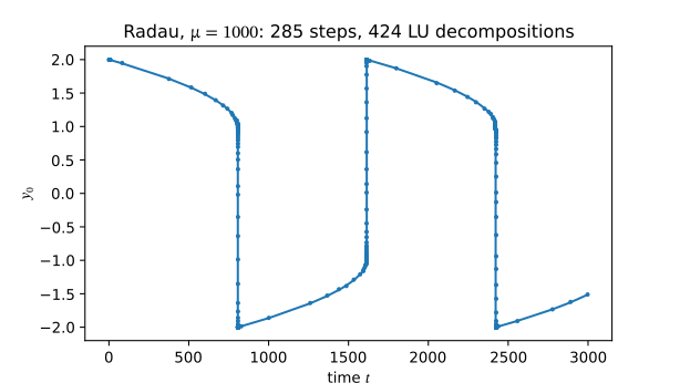
A stiff problem with an event:
const mu = 1000
vdp := func(t float64, y, dydt []float64) {
	dydt[0] = y[1]
	dydt[1] = mu*(1-y[0]*y[0])*y[1] - y[0]
}
cross := integrate.Event{F: func(t float64, y []float64) float64 { return y[0] }}
sol, err := integrate.SolveIVP(vdp, [2]float64{0, 3000}, []float64{2, 0},
	&integrate.IVPOptions{Method: integrate.Radau, Events: []integrate.Event{cross}, DenseOutput: true})
Quadrature with diagnostics:
r, err := integrate.Quad(func(x float64) float64 { return math.Log(x) / math.Sqrt(x) }, 0, 1, nil)
// r.Value = -4 (to 1.7e-14), r.AbsErr = 2.3e-13, r.NEval = 315, err == nil
_, err = integrate.Quad(func(x float64) float64 { return 1 / x }, 0, 1, nil)
// errors.Is(err, integrate.ErrLimit)
The three examples above, drawn with go-plot from the results they return; the markers are the solver’s accepted steps. They were computed on arm64, as the numbers above were. On amd64, where Go does not fuse multiply-adds, the last digits differ: Quad’s error estimate is 1.35e-13 there instead of 2.34e-13, and Radau takes 286 steps instead of 285.
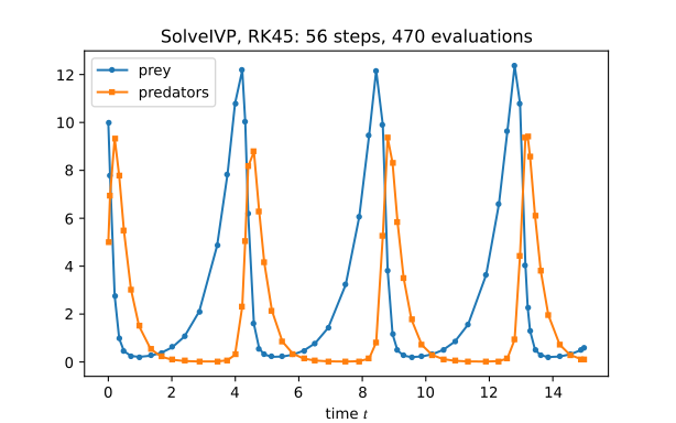
package main

import (
	"fmt"

	"github.com/go-numerics/integrate"
	"github.com/go-plot/plot"
)

func init() { register("lotka", lotka) }

// The README's SolveIVP example: Lotka–Volterra with RK45, the default
// method, and the default tolerances. The markers are the solver's own
// accepted steps, sol.T: no interpolation.
func lotka() *plot.Figure {
	f := func(t float64, y, dydt []float64) {
		dydt[0] = 1.5*y[0] - y[0]*y[1]
		dydt[1] = -3*y[1] + y[0]*y[1]
	}
	sol, err := integrate.SolveIVP(f, [2]float64{0, 15}, []float64{10, 5}, nil)
	if err != nil {
		panic(err)
	}
	prey := make([]float64, len(sol.T))
	predators := make([]float64, len(sol.T))
	for k, y := range sol.Y {
		prey[k], predators[k] = y[0], y[1]
	}
	fig, axs := plot.Subplots(1, 1, plot.FigSize(6.4, 4))
	ax := axs[0][0]
	ax.Plot(sol.T, prey, plot.Marker("o"), plot.MarkerSize(3), plot.Label("prey"))
	ax.Plot(sol.T, predators, plot.Marker("s"), plot.MarkerSize(3), plot.Label("predators"))
	ax.SetTitle(fmt.Sprintf("SolveIVP, RK45: %d steps, %d evaluations", sol.NSteps, sol.NFev))
	ax.SetXLabel(`time $t$`)
	ax.Legend()
	return fig
}
package main

import (
	"fmt"

	"github.com/go-numerics/integrate"
	"github.com/go-plot/plot"
)

func init() { register("vanderpol", vanderpol) }

// The README's stiff example: van der Pol with mu = 1000 over [0, 3000],
// solved with Radau. An explicit method needs millions of steps here.
func vanderpol() *plot.Figure {
	const mu = 1000
	f := func(t float64, y, dydt []float64) {
		dydt[0] = y[1]
		dydt[1] = mu*(1-y[0]*y[0])*y[1] - y[0]
	}
	sol, err := integrate.SolveIVP(f, [2]float64{0, 3000}, []float64{2, 0},
		&integrate.IVPOptions{Method: integrate.Radau})
	if err != nil {
		panic(err)
	}
	y0 := make([]float64, len(sol.T))
	for k, y := range sol.Y {
		y0[k] = y[0]
	}
	fig, axs := plot.Subplots(1, 1, plot.FigSize(6.4, 3.6))
	ax := axs[0][0]
	ax.Plot(sol.T, y0, plot.Marker("o"), plot.MarkerSize(2))
	ax.SetTitle(fmt.Sprintf(`Radau, $\mu = 1000$: %d steps, %d LU decompositions`, sol.NSteps, sol.NLU))
	ax.SetXLabel(`time $t$`)
	ax.SetYLabel(`$y_0$`)
	return fig
}![The integrand log(x)/sqrt(x) on (0, 1], its area shaded, with the value Quad returned](/docs/0.1/images/figures/quad.svg)
package main

import (
	"fmt"
	"math"

	"github.com/go-numerics/integrate"
	"github.com/go-plot/plot"
)

func init() { register("quad", quad) }

// The README's Quad example: an integrand with a singularity at 0, which
// QUADPACK's extrapolation handles. The title prints what Quad returned.
func quad() *plot.Figure {
	f := func(x float64) float64 { return math.Log(x) / math.Sqrt(x) }
	r, err := integrate.Quad(f, 0, 1, nil)
	if err != nil {
		panic(err)
	}
	x := linspace(0.002, 1, 300)
	y := make([]float64, len(x))
	for i, v := range x {
		y[i] = f(v)
	}
	fig, axs := plot.Subplots(1, 1, plot.FigSize(6.4, 4))
	ax := axs[0][0]
	ax.Plot(x, y, plot.Label(`$\log x / \sqrt{x}$`))
	ax.FillBetween(x, y, nil, plot.Alpha(0.3))
	ax.SetYLim(-12, 0.5)
	ax.SetTitle(fmt.Sprintf("Quad: %.12f, error estimate %.1e, %d evaluations", r.Value, r.AbsErr, r.NEval))
	ax.SetXLabel(`$x$`)
	ax.Legend(plot.Loc("lower right"))
	return fig
}
More in example_test.go.
Documentation
- Design — algorithms, sources, where and why the code departs from them, what is not provided.
- Verification — how the results were checked against SciPy, mpmath and the netlib Fortran; the full tables are the quadrature table and the ODE table.
- Performance — timings against SciPy and how they were taken.
Not provided
Complex-valued integrands and states, vectorized right-hand sides, sparse or
banded Jacobians, quad_vec, cubature, tanhsinh, solve_bvp and the
legacy ode class. LSODA is an automatic Runge–Kutta/BDF switch, not a port
of ODEPACK’s Adams/BDF LSODA: same purpose, different evaluation counts (see
design.md).
License
BSD 3-Clause; see LICENSE.
Created on by tannevaled
Modified on by tannevaled