go-numerics is the numerical layer of the Go scientific stack built on go-ndarray: optimisation and root finding, quadrature and ODE solvers, and special functions. Each library ports its reference algorithms — MINPACK, L-BFGS-B, QUADPACK, Radau, BDF, Cephes, Boost.Math — statement by statement, and its tests replay recorded answers: SciPy runs, the netlib Fortran, and mpmath at high precision. No cgo, no assembly.
func main() {
	// Lotka–Volterra: prey y0 and predators y1.
	lotka := func(t float64, y, dydt []float64) {
		dydt[0] = 1.5*y[0] - y[0]*y[1]
		dydt[1] = -3*y[1] + y[0]*y[1]
	}
	sol, err := integrate.SolveIVP(lotka, [2]float64{0, 15}, []float64{10, 5},
		&integrate.IVPOptions{Method: integrate.DOP853, RTol: 1e-10, DenseOutput: true})
	if err != nil {
		panic(err)
	}

	// The dense output between the steps, and the steps themselves.
	t := make([]float64, 600)
	prey, pred := make([]float64, len(t)), make([]float64, len(t))
	for i := range t {
		t[i] = 15 * float64(i) / float64(len(t)-1)
		y := sol.Sol.Eval(t[i])
		prey[i], pred[i] = y[0], y[1]
	}
	stepPrey := make([]float64, len(sol.T))
	for k, y := range sol.Y {
		stepPrey[k] = y[0]
	}

	fig, axs := plot.Subplots(1, 1, plot.FigSize(6.4, 4))
	ax := axs[0][0]
	ax.Plot(t, prey, plot.Label("prey"))
	ax.Plot(t, pred, plot.Label("predators"), plot.LineStyle("--"))
	ax.Plot(sol.T, stepPrey, plot.Marker("o"), plot.LineStyle("None"),
		plot.MarkerSize(3), plot.Color("C0"), plot.Label("accepted steps"))
	ax.SetTitle(fmt.Sprintf("DOP853, rtol 1e-10: %d steps, %d evaluations", sol.NSteps, sol.NFev))
	ax.SetYLim(-0.5, 19)
	ax.SetXLabel(`time $t$`)
	ax.Legend(plot.Loc("upper left"))
	if err := fig.SaveSVG(os.Stdout); err != nil {
		panic(err)
	}
}
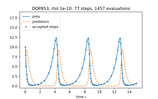
integrate solves Lotka–Volterra with DOP853 at a relative tolerance of 1e-10; the lines are its dense output, the dots its accepted steps, and the title prints the counts it returned. go-plot drew the SVG. The CI runs the program again and fails if one byte of the figure differs.
A census of 339 scientific notebooks set optimize's order — minimize, minimize_scalar, scalar roots, root, least_squares and curve_fit, linprog — and integrate and special cover quad, solve_ivp and the functions every statistic is computed with. Each Go function names the reference call it corresponds to.
Nelder–Mead, Powell, CG, BFGS, Newton-CG and L-BFGS-B; Brent, Ridder and Newton for scalar roots; MINPACK's hybrid method for systems.
Levenberg–Marquardt and trust-region reflective with bounds and robust losses; CurveFit with the parameter covariance; linear programming with duals.
QUADPACK ported from the netlib Fortran: singularities, infinite ranges, oscillatory and algebraic weights, Cauchy principal values; double, triple and N-dimensional integrals.
RK45, RK23, DOP853, Radau and BDF with events and dense output, and an automatic Runge–Kutta/BDF switch for problems that turn stiff.
Gamma, beta, erf and the normal distribution, incomplete gamma and beta and their inverses, Bessel functions of real order, zeta, elliptic integrals.
Curve-fit data, covariances, LP matrices and ODE solutions are *ndarray.Array; special/nd applies a function element-wise with broadcasting, across cores.
No cgo, no assembly. CI runs the tests on amd64 and arm64 and under emulation on riscv64, loong64, ppc64le and s390x.
Every repository of the organization. Ported code keeps its attribution in place.
The fixtures are written by scripts that call the reference — SciPy 1.18.1, the netlib Fortran, mpmath at 192 and 320 bits — committed, and compared in the tests. What differs, and why, is in each library's documentation.
116 of 124 fixture integrals take exactly SciPy 1.18.1’s subdivision path: the same evaluation count, the value to 1e-12. Three of the others are where SciPy’s C translation departs from the netlib Fortran, and this port agrees with the Fortran. (integrate)
110 of 120 solve_ivp runs of the ported methods take exactly SciPy’s steps: the same function evaluations, steps, Jacobians and LU decompositions. (integrate)
On the arithmetic-only problems, 36 of 38 Minimize runs take SciPy’s exact path (identical nit, nfev, njev); L-BFGS-B is bit-identical to SciPy’s C code built with sequential BLAS. (optimize)
Root/Fsolve: 23 of 23 runs with identical counts, status and message, x bit-identical. Linprog: 46 of 46 statuses against HiGHS, objective error at most 1.8e-15 with the simplex. (optimize)
About 250 000 points in 419 regions over 62 functions, against mpmath at high precision: the maximum error is at or below SciPy’s in 418 regions, and the one exception is a tie at 1.05 ulp. (special)
One thing broken at a time — a BFGS term dropped, a sign flipped in Moré–Thuente, a Kronrod weight nudged by 1e-6, a coefficient of the Γ(1+t) core moved by 1.5 ulp — and each break makes the suite fail. (optimize, integrate, special)
Medians of interleaved Go and SciPy 1.18.1 runs on a shared, loaded 16-core Apple M4 Max, from each library's docs/perf.md. SciPy's numbers include its Python callbacks, which is most of its time on small problems; the documentation gives them without, too. The rows in the library's colour are where SciPy is faster.
| case | go-numerics | SciPy 1.18.1 | SciPy / Go |
|---|---|---|---|
| Brentq, x³ − 2x − 5 (optimize) | 0.27 µs | 8.6 µs | 32× |
| Rosenbrock n=100, BFGS (optimize) | 14.8 ms | 87.9 ms | 5.9× |
| Rosenbrock n=100, L-BFGS-B (optimize) | 6.36 ms | 23.2 ms | 3.7× |
| curve_fit, 10⁴ points, LM (optimize) | 4.13 ms | 2.78 ms | 0.67× |
| curve_fit, 10⁴ points, TRF (optimize) | 5.97 ms | 4.61 ms | 0.77× |
| ∫₀¹ log x/√x, Quad (integrate) | 4.7 µs | 30.1 µs | 6× |
| Lotka–Volterra, RK45 (integrate) | 18.1 µs | 1.67 ms | 92× |
| Van der Pol μ=1000, Radau (integrate) | 199.9 µs | 37.72 ms | 189× |
| Gamma, 10⁶ points, one thread (special) | 45.5 ns/elem | 13.4 ns/elem | 0.30× |
Gamma, 10⁶ points, special/nd on 16 cores | 6.4 ns/elem | 13.4 ns/elem | 2.1× |
Minimisation (Nelder–Mead, Powell, CG, BFGS, Newton-CG, L-BFGS-B), scalar and system roots (Brent, MINPACK hybrd), nonlinear least squares (Levenberg–Marquardt, trust-region reflective, robust losses), curve fitting with covariance, linear programming (simplex, interior point).
Adaptive quadrature ported from the netlib QUADPACK, fixed and sample rules, double, triple and N-dimensional integrals, and initial value problems with RK45, RK23, DOP853, Radau, BDF and automatic stiffness switching, with events and dense output.
Gamma, beta, error and normal functions, incomplete gamma and beta and their inverses, Bessel, zeta, combinatorics, logistic helpers and complete elliptic integrals, each measured in ULPs against mpmath; special/nd applies them element-wise to go-ndarray arrays, across cores.
The documentation (Hugo + Hextra): one section per library, made of its own README, design, verification, accuracy and performance documents, with figures each library computed. Source →
Logos and icons for the organization, in SVG / PNG / JPG / ICO / ICNS across colour, white and black variants.
go-numerics computes on the arrays of go-ndarray, its results plot with go-plot, and a go-notebook cell can use all three. What is not in v0.1 yet — constrained minimisers, global optimisers, boundary value problems, complex-valued integrands — is listed in the documentation.
Read the source on GitHub → go-numerics